| TLA | Logic | Symbol | Variants |
|---|---|---|---|
| PRP | PRoPositional | fof | |
| CNF | Clause Normal Form | cnf | |
| FOF | First-Order Form | fof | |
| TFF | Typed First-order Form | tff | TF0 - monomorphic; TF1 - polymorphic |
| TXF | Typed eXtended first-order Form | tff | TX0 - monomorphic; TX1 - polymorphic |
| THF | Typed Higher-order Form | thf | TH0 - monomorphic; TH1 - polymorphic |
| DHF | Dependently typed Higher-order Form | thf | DH0 - monomorphic; DH1 - polymorphic |
| NXF | Non-classical typed eXtended first-order Form | tff | TX0 - monomorphic; TX1 - polymorphic |
| NHF | Non-classical typed Higher-order Form | thf | NH0 - monomorphic; NH1 - polymorphic |
| NTF | Non-classical Typed Form | - | NXF and NHF |
TPTP problems and TSTP solutions are built from annotated formulae of the form
language(name,role,formula,source,useful_info).
The languages supported are cnf, fof, tff, and thf.
The role gives the user semantics of the formula, one of
axiom, hypothesis, definition, assumption,
lemma, theorem, corollary, conjecture,
negated_conjecture, plain, type, interpretation,
logic, and
unknown.
The useful_info field of an annotated formula is optional, and if it is not used then
the source field becomes optional.
The source field is used to record where the annotated formula came from, and is most commonly a
file record or an inference record.
A file record stores the name of the file from which the annotated formula was read, and
optionally the name of the annotated formula as it occurs in that file - this might be different
from the name of the annotated formula itself, e.g., if an ATP systems reads an annotated formula,
renames it, and then prints it out.
An inference record stores information about an inferred formula.
The useful_info field of an annotated formula is a list of arbitrary useful information
formatted as Prolog terms, as required for user applications.
Logical Formulae
The logical connectives in the classical TPTP languages are
!>, ?*, @+, @-, ^, !, ?, @,
~, |, &, =>, <=, <=>, and
<~>, for Pi, Sigma, choice (indefinite description), definite description, lambda
abstraction, universal quantification, existential quantification, function application, negation,
disjunction, conjunction, implication, reverse implication, equivalence, and non-equivalence (XOR).
Equality and inequality are expressed as the infix predicates = and !=.
Quantified formulae are written in the form
Types
Defined Symbols
Conditional and Let Expressions
Examples
Subtypes
Defined atomic types
User atomic type declarations:
Defined functions and predicates
Function and predicate type declarations
Annotated Formulae
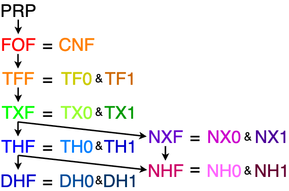
The TPTP contains problems in first-order (FOF) and clause normal form (CNF),
monomorphic and polymorphic typed first-order form (TFF, which includes the extended first-order
form (TXF)), monomorphic and polymorphic typed higher-order form (THF),
dependently typed monomorphic and polymorphic typed higher-order form (DHF),
and non-classical typed first-order (NXF) and higher-order (NHF) forms.
Interpreted arithmetic types and symbols are supported in all the typed logics.
In a formula, terms and atoms follow Prolog conventions - functions and predicates start
with a lowercase letter or are 'single quoted', and variables start with an
uppercase letter.
Symbols may be overloaded with different arity signatures, and are treated as different symbols.
The language also supports interpreted symbols that are either defined symbols that start with
a $, or are composed of non-alphabetic characters.
Defined symbols come in two varieties: TPTP defined predicates and functors, whose
interpretation is specified by the TPTP language, and system defined predicates and
functors, whose interpretation is ATP system specific.
The defined predicates and functors recognized so far are listed below.
Quantifier [Variables] : Formula
In all except the CNF language, every variable in a Formula must be bound by a
preceding quantification with adequate scope.
Negation has higher precedence than quantification, which in turn has
higher precedence than the binary connectives.
No precedence is specified between the binary connectives; brackets are
used to ensure the correct association.
See the section on
non-classical logics for information about the non-classical connectives.
The typed languages (TFF, TXF, THF, DHF, NXF, NHF) support types and type declarations
(all the details are in the section on types and type declarations).
Symbols are declared before their use, with type signatures that specify the types of their
arguments and result.
Two TPTP defined types are available, $i for individuals, and $o for booleans.
User defined types can be introduced as being of the "type" $tType.
In the first-order languages, a signature of the form
(t1 * ... * tn) > r
is the type of an n-ary symbol, where the i-th argument is of type ti and the
result type is r.
If r is $o then the symbol is a predicate.
Variables are given their type by a :type suffix.
Equality is ad hoc polymorphic over all types.
A useful feature of TFF is default typing for symbols that are not explicitly declared:
predicates default to ($i,...,$i) > $o, and functions default to
($i,...,$i) > $i.
This allows TFF to effectively degenerate to untyped FOF.
The typed extended first-order form (TXF) augments TFF with FOOL constructs:
formulae of type $o as terms; variables of type $o as formulae; tuples;
conditional (if-then-else) expressions; and let (let-defn-in) expressions.
The typed higher-order form (THF) includes type declarations in curried form, lambda-terms with
a binder symbol ^ for lambda, explicit application with @, and quantification
over variables of any type.
A curried type signature has the form
t1 > ... > tn > r.
THF does not admit default typing - all symbol types must be declared before use.
The polymorphic languages use a !> to quantify over types, producing types signatures
of the form
!> [T:$tType] : (t1 * ... * tn) > r
and
!> [T:$tType] : t1 > ... > tn > r.
where any ti or r can be the type
T.
When using polymorphic symbols the concrete type(s) must be provided as the first arguments in
the use.
The defined symbols are:
The THF and TXF languages have conditional and let expressions.
%----The constant function using A from 'outside' and B from 'inside'. B
%----is required in the use of const, but not A.
tff(let_polymorphic_both_types, axiom,
    !>[A: $tType] :
      $let(
        const : !>[B: $tType] : (A * B) > A,
        const(B, X, Y) := X),
        ... ).
No extra type arguments are needed when using such $let-defined symbols.
An example CNF problem is
PUZ003-1.
An example FOF problem is
PUZ001+1.
An example TFF problem is
PUZ031_1.
An example TXF problem is
PUZ081_8.
An example THF problem is
PUZ081^1.
An example DHF problem is
DAT346^1.
An example NXF problem is
PUZ001_10.
An example NHF problem is
PHI003^8.
The Type System
A high-level overview is in the section on annotated formulae.
None of the type systems offer subtypes, despite the subtype symbol << being part
of the THF and
TFF languages.
I tried to convince the ATP system developers it would be useful, but they cried crocodile tears.
Here's an example of what was planned:
    tff(food_type,type, food: $tType).

    tff(fruit_type,type, fruit: $tType).

    tff(vegetable_type,type, vegetable: $tType).

    tff(fruit_is_food,type,
        fruit << food ).

    tff(vegetable_is_food,type,
        vegetable << food ).

    tff(apple_decl,type, apple: fruit).

    tff(potatoe_decl,type, potatoe: vegetable).
All subtypes of an atomic type are disjoint, i.e., it is implicit that apple != potatoe.
The Typed First-order Monomorphic Type System (TF0 and TX0)
Refer to
[SS+12] (TF0) and
[SK18] (TX0)
for more details on type checking and semantics, and much more.
The atomic types $i (individuals), $o (Booleans), and $tType are
defined.
($tType is the "type" of atomic types - it is not really a type, and in other places this
is known as the "kind" of atomic types.
See below for motivation for its existence and usage.)
Other defined atomic types are associated with specific theories.
In particular, $int, $rat, and $real are types for
arithmetic.
The type $i of individuals is predefined but has no peculiar semantics, whereas the
arithmetic types $int, $rat, and $real are modeled by ℤ, ℚ,
and ℝ, respectively.
User atomic types are declared in advance of use, to be of "type" $tType.
Example:
    tff(food_type,type,
        food: $tType ).

    tff(fruit_type,type,
        fruit: $tType ).

    tff(list_type,type,
        list: $tType ).
Defined functions and predicates have preassigned types.
Every function and predicate symbol has maximally one declared type.
Example:
    tff(cons_type,type,
        cons: (fruit * list) > list   ).

    tff(is_empty_type,type,
        isEmpty: list > $o   ).
The argument types must be atomic, and cannot be $o in TFF, but can be $o in TXF.
The range type of a function must be atomic, and cannot be $o.
The range type of a predicate is $o.
Currying is not possible in TFF or TXF, i.e., the first example above cannot be written
cons: fruit > list > list
(currying is used in THF and DHF).
If a symbol's type is declared more than once, and the types are not the same, that's an error.
Every variable is given an atomic type at quantification time. Example:
    tff(list_not_empty,axiom,
        ! [X: fruit,Xs: list] : ~isEmpty(cons(X,Xs))   ).
Implicit typing for functions and predicates
If a symbol is used and its type has not been declared, then default types are assumed.
The Typed First-order Polymorphic Type System (TF1 and TX1)
Refer to
[BP13]
for more details on type checking and semantics, and much more.
The TF1 polymorphic type system extends the monomorphic type system with rank-1 polymorphism. Syntactically, the types, terms, and formulas of TF1 are analogous to those of TF0, except that function and predicate symbols can be declared to be polymorphic, types can contain type variables, and n-ary type constructors are allowed. Type variables in type signatures and formulas are explicitly bound. Instances of polymorphic symbols are specified by explicit type arguments, rather than inferred.
Types and type signatures
The types of TF1 are built from type variables and type constructors
of fixed arities.
A type is polymorphic if it contains type variables (otherwise, it is monomorphic).
Polymorphic type signatures are of the form:
!>[α1 : $tType, ..., αn : $tType]: ς
for n > 0, where α1, ..., αn are distinct type variables
and ς is a monomorphic type.
The binder !> denotes universal quantification.
Type declarations
Type constructors can be declared, e.g., the following declarations introduce a type constant
bird, a unary type constructor list, and a binary type constructor map:
    tff(bird_t, type, bird: $tType).
    tff(list_t, type, list: $tType > $tType).
    tff(map_t, type, map: ($tType * $tType) > $tType).
Every type variable must be bound by a !>-binder.
The following declarations introduce a polymorphic predicate is_empty, and a pair of
polymorphic functions cons and lookup:
    tff(is_empty_t, type, is_empty : !>[A : $tType]: (list(A) > $o)).
    tff(cons_t, type, cons : !>[A : $tType]: ((A * list(A)) > list(A))).
    tff(lookup_t, type, lookup : !>[A : $tType, B : $tType]: ((map(A, B) * A) > B)).
Using symbols with a polymorphic type
Every use of a polymorphic symbol must explicitly specify the type instance.
A function or predicate symbol with a type signature
!>[α1$: $tType, ..., αm : $tType]:
((τ1 * ... * τn) > υ)
must be applied to m type arguments and n term arguments.
Given the above signatures, the term lookup($int, list(A), M, 2) and the atom
is_empty($i, cons($i, X, nil($i))) are well-formed and contain free occurrences of
the type variable A and the term variable X, respectively.
As TF1 is restricted to rank-1 polymorphism, type variables can be instantiated with only
concrete types.
In particular, $o, $tType, and !>-binders cannot occur in type
arguments of polymorphic symbols.
Every variable in a TF1 formula must be bound. In particular, every type variable in a TF1 formula must be bound with the pseudotype $tType:
    tff(bird_list_not_empty, axiom,
        ![B : bird, Bs : list(bird)]: ~ is_empty(bird, cons(bird, B, Bs))).

    tff(lookup_update_same, axiom,
        ! [A : $tType, B : $tType, M : map(A, B), K : A, V : B]:
          lookup(A, B, update(A, B, M, K, V), K) = V).
Universal and existential quantifiers over type variables may not occur in the scope of a
quantifier over a term variable (as is possible in dependent types).
Example
An example TF1 problem is
PUZ139_1.
The Typed Higher-order Monomorphic Type System (TH0)
Refer to
[SB10]
for more details on type checking and semantics, and much more.
The TH0 monomorphic type system lifts the TF0 type system to simply typed λ-calculus, with Henkin semantics (i.e., including Boolean and functional extensionality) and choice. Type signatures are curried, and variables can have function types. Example:
    thf(mix_type,type,
        mix: beverage > syrup > beverage ).

    thf(mixed_coffee,conjecture,
        ? [Mixture: beverage > syrup > beverage] :
        ! [S: syrup] :
          ( ( Mixture @ coffee @ S ) = coffee ) ).
An example TH0 problem is PUZ140^1.
The Typed Higher-order Polymorphic Type System (TH1)
Refer to
[KSR16]
for more details on type checking and semantics, and much more.
The TH1 polymorphic type system combines the polymorphic features of TF1/TX1 with the higher-order
features of TH0.
Example:
    thf(list,type, list: $tType > $tType ).

    thf(nil,type, nil: !>[A: $tType] : ( list @ A ) ).

    thf(append,type, append: !>[A: $tType] : ( ( list @ A ) > ( list @ A ) > ( list @ A ) ) ).

    thf(append_nil,axiom,
        ! [A: $tType,L: list @ A] :
          ( ( append @ A @ ( nil @ A ) @ L ) = L ) ).
TH1 has five additional polymorphic constants: !! for Π (universal quantification), ?? for Σ (existential quantification), @@+ for ε (indefinite description, aka choice), @@- for ι (definite description), and @= (equality). The type of the first four is !>[A: $tType] : (A > $o) > $o, and the type of @= is !>[A: $tType]: (A > A) > $o. When used they must be instantiated by applying them to a type argument. Example:
    thf(eps,type, eps: ( $i > $o ) > $i ).

    thf(choiceax,axiom,
        ! [P: $i > $o] :
          ( ? [X: $i] : ( P @ X )
         => ( P @ ( eps @ P ) ) ) ).

    thf(conj,conjecture,
        ( ( ^ [P: $i > $o] : ( P @ ( eps @ P ) ) )
        = ( ^ [P: $i > $o] : ( ?? @ $i @ P ) ) ) ).

    thf(bird_type,type, bird: $tType).

    thf(tweety_decl,type, tweety: bird).

    thf(some_tweety,axiom,
        ? [B: bird] : ( (@= @ bird) @ tweety @ B ) ).
An example TH1 problem is DAT434^1.
The Dependently Typed Higher-order Type System (DH0 and DH1)
Refer to
[RK+25]
for more details on type checking and semantics, and much more.
The DH0 and DH1 type systems add dependent types, i.e., types that take term arguments, to TH0 and TH1. As such they are classical and extensional type theories. The !> binder used for TF1 and TH1 polymorphism is reused to specify the term typess on which a type depends. Example:
    thf(elem_type,type, elem: $tType ).

    thf(nat_type,type, nat: $tType ).

    thf(zero_type,type, zero: nat ).

    thf(suc_type,type, suc: nat > nat ).

    thf(plus_type,type, plus: nat > nat > nat ).

    thf(list_type,type, list: nat > $tType ).

    thf(nil_type,type, nil: list @ zero ).

    thf(cons_type,type, cons:
        !>[N: nat] : (elem > (list @ N) > (list @ (suc @ N))) ).

    thf(app_type,type, app:
        !>[N: nat,M: nat] : ((list @ N) > (list @ M) > (list @ (plus @ N @ M))) ).
The application operator @ is used to instantiate the terms to the dependent type.
With polymorphic types, the variable list is prepended with the type variables.
Example:
    thf(ax1,axiom,
        ! [N: nat] : ((plus @ zero @ N) = N) ).

    thf(ax2,axiom,
        ! [N: nat,X: list @ N] : ((app @ zero @ N @ nil @ X) = X) ).

    thf(list_app_assoc_base,conjecture,
        ! [M2: nat,L2: list @ M2,M3: nat,L3: list @ M3] :
          ( ( app @ zero @ ( plus @ M2 @ M3 ) @ nil @ ( app @ M2 @ M3 @ L2 @ L3 ) )
          = ( app @ ( plus @ zero @ M2 ) @ M3 @ ( app @ zero @ M2 @ nil @ L2 ) @ L3 ) ) ).
An example DH0 problem is
DAT346^1.
An example DH1 problem is
DAT342^1.
The Arithmetic System
Arithmetic must be done in the context of the THF or TFF types logics, which
support the predefined atomic numeric types
$int, $rat, and $real.
Using THF or TFF enforces semantics that separate
$int from $rat from $real from $i from $o.
The numbers are unbounded, and the reals of infinite precision (rather
than some specific implementation such as 32 bit 2's complement integer, or
IEEE floating point).
Systems that implement limited arithmetic must halt in an
SZS error state if they hit overflow.
The following interpreted predicates and interpreted functions are defined. The symbols are overloaded (i.e., ad-hoc polymorphic) for the provided type signatures.
| Symbol | Types | Operation | Comments, examples - |
|---|---|---|---|
| $int | $tType | The type of integers | 123, -123<integer> ::- (<signed_integer>|<unsigned_integer>) <signed_integer> ::- <sign><unsigned_integer> <unsigned_integer> ::- <decimal> <decimal> ::- (<zero_numeric>|<positive_decimal>) <positive_decimal> ::- <non_zero_numeric><numeric>* <sign> ::: [+-] <zero_numeric> ::: [0] <non_zero_numeric> ::: [1-9] <numeric> ::: [0-9] |
| $rat | $tType | The type of rationals | 123/456, -123/456, +123/456
<rational> ::- (<signed_rational>|<unsigned_rational>) <signed_rational> ::- <sign><unsigned_rational> <unsigned_rational> ::- <decimal><slash><positive_decimal> <slash> ::: [/] |
| $real | $tType | The type of reals | 123.456, -123.456, 123.456E789, 123.456e789, -123.456E789, 123.456E-789, -123.456E-789 <real> ::- (<signed_real>|<unsigned_real>) <signed_real> ::- <sign><unsigned_real> <unsigned_real> ::- (<decimal_fraction>|<decimal_exponent>) <decimal_exponent> ::- (<decimal>|<decimal_fraction>)<exponent><decimal> <decimal_fraction> ::- <decimal><dot_decimal> <dot_decimal> ::- <dot><numeric><numeric>* <dot> ::: [.] <exponent> ::: [Ee] |
| = (infix) |
($int * $int) > $o ($rat * $rat) > $o ($real * $real) > $o | Comparison of two numbers. | The numbers must be the same atomic type (see the type system). |
| $less/2 |
($int * $int) > $o ($rat * $rat) > $o ($real * $real) > $o | Less-than comparison of two numbers. | $less, $lesseq, $greater,
and $greatereq are related by ! [X,Y] : ( $lesseq(X,Y) <=> ( $less(X,Y) | X = Y ) ) ! [X,Y] : ( $greater(X,Y) <=> $less(Y,X) ) ! [X,Y] : ( $greatereq(X,Y) <=> $lesseq(Y,X) ) i.e, only $less and equality need to be implemented to get all four relational operators. |
| $lesseq/2 |
($int * $int) > $o ($rat * $rat) > $o ($real * $real) > $o | Less-than-or-equal-to comparison of two numbers. | |
| $greater/2 |
($int * $int) > $o ($rat * $rat) > $o ($real * $real) > $o | Greater-than comparison of two numbers. | |
| $greatereq/2 |
($int * $int) > $o ($rat * $rat) > $o ($real * $real) > $o | Greater-than-or-equal-to comparison of two numbers. | |
| $uminus/1 |
$int > $int $rat > $rat $real > $real | Unary minus of a number. | $uminus, $sum, and $difference are
related by ! [X,Y] : $difference(X,Y) = $sum(X,$uminus(Y)) i.e, only $uminus and $sum need to be implemented to get all three additive operators. |
| $sum/2 |
($int * $int) > $int ($rat * $rat) > $rat ($real * $real) > $real | Sum of two numbers. | |
| $difference/2 |
($int * $int) > $int ($rat * $rat) > $rat ($real * $real) > $real | Difference between two numbers. | |
| $product/2 |
($int * $int) > $int ($rat * $rat) > $rat ($real * $real) > $real | Product of two numbers. | |
| $quotient/2 |
($int * $int) > $rat ($rat * $rat) > $rat ($real * $real) > $real | Exact quotient of two numbers of the same type. | For non-zero divisors, the result can be computed.
For zero divisors the result is not specified.
In practice, if an ATP system does not "know" that the divisor
is non-zero, it should simply not evaluate the $quotient.
Users should always guard their use of $quotient using
inequality, e.g., ! [X: $real] : ( X != 0.0 => p($quotient(5.0,X)) ) For $rat or $real operands the result is the same type. For $int operands the result is $rat; the result might be simplied. |
| $quotient_e/2, $quotient_t/2, $quotient_f/2 |
($int * $int) > $int ($rat * $rat) > $rat ($real * $real) > $real | Integral quotient of two numbers. | The three variants use different rounding to an integral result:
|
| $remainder_e/2, $remainder_t/2, $remainder_f/2 |
($int * $int) > $int ($rat * $rat) > $rat ($real * $real) > $real | Remainder after integral division of two numbers. | For τ ∈ {$int,$rat,
$real}, ρ ∈ {e,
t,f}, $quotient_ρ and
$remainder_ρ are related by ! [N:τ,D:τ] : $sum($product($quotient_ρ(N,D),D),$remainder_ρ(N,D)) = N For zero divisors the result is not specified. |
| $floor/1 |
$int > $int $rat > $rat $real > $real | Floor of a number. | The largest integral value (in the type of the argument) not greater than the argument (i.e., ! [X] : ($is_int($floor(X)))). |
| $ceiling/1 |
$int > $int $rat > $rat $real > $real | Ceiling of a number. | The smallest integral value (in the type of the argument) not less than the argument (i.e., ! [X] : ($is_int($ceiling(X)))). |
| $truncate/1 |
$int > $int $rat > $rat $real > $real | Truncation of a number. | The nearest integral value (in the type of the argument) with magnitude not greater than the absolute value of the argument (i.e., ! [X] : ($is_int($truncate(X)))). |
| $round/1 |
$int > $int $rat > $rat $real > $real | Rounding of a number. | The nearest integral value (in the type of the argument) to the argument (i.e., ! [X] : ($is_int($rount(X)))). If the argument is halfway between two integral values, the nearest even integral value to the argument. |
| $abs/1 |
$int > $int $rat > $rat $real > $real | Absolute value of a number. | $abs is related to other operators by
    ! [X] :
      ( ( $greatereq(X,0)
       => $abs(X) = X )
      & ( $less(X,0)
       => $abs(X) = $uminus(X) ) )
|
| $is_int/1 |
$int > $o $rat > $o $real > $o | Test for coincidence with an $int value. | |
| $is_rat/1 |
$int > $o $rat > $o $real > $o | Test for coincidence with a $rat value. | |
| $to_int/1 |
$int > $int $rat > $int $real > $int | Coercion of a number to $int. | The largest $int not greater than the argument; the argument effectively gets truncated before conversion: ! [X] : ($to_int($truncate(X)) = $to_int(X)). If applied to an argument of type $int, this is the identity function. |
| $to_rat/1 |
$int > $rat $rat > $rat $real > $rat | Coercion of a number to $rat. | This function is not fully specified.
If applied to an argument of type $int, the result is the argument over
1.
If applied to an argument of type $rat, this is the identity function.
If applied to an argument of type $real that is (known to be) rational, the
result is the $rat value.
For other reals the result is not specified.
In practice, if an ATP system does not "know" that the argument
is rational, it should simply not evaluate the $to_rat.
Users should always guard their use of $to_rat using
$is_rat, e.g., ! [X: $real] : ( $is_rat(X) => p($to_rat(X)) ) |
| $to_real/1 |
$int > $real $rat > $real $real > $real | Coercion of a number to $real. | If applied to an argument of type $real, this is the identity function. |
The extent to which ATP systems are able to work with the arithmetic
predicates and functions can vary, from a simple ability to evaluate ground
terms, e.g., $sum(2,3) can be evaluated to 5, through
an ability to instantiate variables in equations involving such functions,
e.g., $product(2,$uminus(X)) = $uminus($sum(X,2))
can instantiate X to 2, to extensive algebraic manipulation
capability.
The syntax does not axiomatize arithmetic theory, but may be used to write
axioms of the theory.
In NXF the non-classical connectives are applied in a mixed
higher-order-applied/first-order-functional style, with the connectives applied using @
to a ()ed list of arguments.
In NHF the non-classical connectives are applied using @ in usual higher-order style with
curried function applications.
There are also short form unary connectives for unparameterised {$box} and
{$dia}, applied directly like negation: [.] and <.>, e.g.,
{$box} @ (p) can be
written [.] p.
Short forms and long forms can be used together, e.g., it's OK to use {$necessary} and
[.] in the same problem or formula.
Full specification of the connectives and their use in formulae is in the BNF
starting at
<nxf_atom> and
<thf_defined_atomic>.
Semantics Specification
A semantic specification changes the meaning of things such as the boolean type $o,
universal quantification with !, etc - their existing meaning in classical logic should
not be confused with the meaning in the declared logic.
For plain $modal and all the *_modal logics the properties that may be
specified are $domains, $designation, $terms, and $modalities.
For $temporal_instant the properties are the $domains, $designation,
and $terms of the modal logic, $modalities with different possible values,
and another property $time.
The formulae of a problem can be either local (true in the current world) or global (true in all
worlds).
By default, formulae with the roles hypothesis and conjecture are local, and
all others are global.
These defaults can be overridden by adding a subrole, e.g., axiom-$local,
conjecture-$global.
The Non-classical Logics
The TPTP recognizes several normal modal logics, and one temporal logic.
Each logic has a defined name:
Connectives
The non-classical connectives of NTF have the form {$name}.
For the logics recognized by the TPTP the connectives are:
(System names may also be used for user-defined connectives, e.g.,
{$$canadian_conditional}, thus allowing use of the TPTP syntax when experimenting with
logics that have not yet been formalized in the TPTP.)
A connective can be parameterized to reflect more complex non-classical connectives.
The form is
{$name(param1,param2,param2)}.
If the connective is indexed the index is given as the first parameter prefixed with a #,
e.g., {$knows(#manuel)} @ (nothing)},
so that the connective is {$knows(#manuel)} (and not the connective {$knows}
applied to the index #manuel).
All other parameters are key-value assignments, e.g., to list the agents of common knowledge the
form might be {$common($agents:=[alice,bob,claire])}.
An annotated formula with the role logic is used to specify the semantics of formulae.
The semantic specification typically comes first in a file.
A semantic specification consists of the defined name of the logic followed by
== and a list of properties value assignments.
Each specification is the property name, followed by == and either a value or a tuple
of specification details.
If the first element of a list of details is a value, that is the default value for all cases
that are not specified in the rest of the list.
Each detail after the optional default value is the name of a relevant part of the vocabulary of
the problem, followed by == and a value for that named part.
The BNF grammar is
here.
The grammar is not very restrictive on purpose, to enable working with other logics as well.
It is possible to create a lot of nonsense specifications, and to say the same thing in different
meaningful ways.
A tool to check the sanity of a specification is available.
Sys ∈ { K,KB,K4,K5,K45,KB5,D,DB,D4,D5,D45,M,B,S4,S5,S5U }
Axi ∈ { K,M,B,D,4,5,CD,BoxM,C4,C }
Axi ∈ { K,M,B,D,4,5 },
Tmi ∈ { +,- },
Pi
∈ { $reflexivity, $irreflexivity, $transitivity, $asymmetry, $anti_symmetry,
$linearity, $forward_linearity, $backward_linearity, $beginning, $end, $no_beginning,
$no_end, $density, $forward_discreteness, $backward_discreteness }
The TPTP Language BNF
% v9.3.0.1 - Removed fi_ roles, added datatype, codatatype, datatype_constructor, and
% codatatype_constructor.
%--------------------------------------------------------------------------------------------------
%----README ... this header provides important meta- and usage information
%----
%----Intended uses of the various parts of the TPTP syntax are explained in the TPTP technical
%----manual, linked from www.tptp.org.
%----
%----Four kinds of separators are used, to indicate different types of rules:
%---- ::= is used for regular grammar rules, for syntactic parsing.
%---- :== is used for semantic grammar rules. These define specific values that make semantic
%---- sense when more general syntactic rules apply.
%---- ::- is used for rules that produce tokens.
%---- ::: is used for rules that define character classes used in the construction of tokens.
%----
%----White space may occur between any two tokens. White space is not specified in the grammar, but
%----there are some restrictions to ensure that the grammar is compatible with standard Prolog: a
%----<TPTP_file> should be readable with read/1.
%----
%----The syntax of comments is defined by the <comment> rule. Comments may occur between any two
%----tokens, but do not act as white space. Comments will normally be discarded at the lexical
%----level, but may be processed by systems that understand them (e.g., if the system comment
%----convention is followed).
%----
%----Multiple languages are defined. Depending on your need, you can implement just the one(s) you
%----need. The common rules for atoms, terms, etc, come after the definitions of the languages, and
%----mostly all needed for all the languages.
%--------------------------------------------------------------------------------------------------
%----Files. Empty file is OK.
<TPTP_file> ::= <TPTP_input>*
<TPTP_input> ::= <annotated_formula> | <include>
%----Formula records
<annotated_formula> ::= <thf_annotated> | <tff_annotated> | <tcf_annotated> | <fof_annotated> |
<cnf_annotated> | <tpi_annotated>
%----Future languages may include ... english | efof | tfof | mathml | ...
<tpi_annotated> ::= tpi(<name>,<formula_role>,<tpi_formula><annotations>).
<tpi_formula> ::= <fof_formula>
<thf_annotated> ::= thf(<name>,<formula_role>,<thf_formula><annotations>).
<tff_annotated> ::= tff(<name>,<formula_role>,<tff_formula><annotations>).
<tcf_annotated> ::= tcf(<name>,<formula_role>,<tcf_formula><annotations>).
<fof_annotated> ::= fof(<name>,<formula_role>,<fof_formula><annotations>).
<cnf_annotated> ::= cnf(<name>,<formula_role>,<cnf_formula><annotations>).
<annotations> ::= ,<source><optional_info> | <nothing>
%----In derivations the annotated formulae names must be unique, so that parent references (see
%----<inference_record>) are unambiguous.
%----Types for problems.
%----Note: The previous <source_type> from ...
%---- <formula_role> ::= <user_role>-<source>
%----... is now gone. Parsers may choose to be tolerant of it for backwards compatibility.
<formula_role> ::= <lower_word> | <lower_word>-<general_term>
<formula_role> :== axiom | hypothesis | definition | assumption | lemma | theorem |
corollary | conjecture | negated_conjecture | plain | type |
interpretation | unknown
%----"axiom"s are accepted, without proof. There is no guarantee that the axioms of a problem are
%----consistent. "hypothesis"s are assumed to be true for a particular problem, and are used like
%----"axiom"s. "definition"s are intended to define symbols. They are either universally quantified
%----equations, or universally quantified equivalences with an atomic lefthand side. They can be
%----treated like "axiom"s. "assumption"s can be used like axioms, but must be discharged before a
%----derivation is complete. "lemma"s and "theorem"s have been proven from the "axiom"s. They can
%----be used like "axiom"s in problems, and a problem containing a non-redundant "lemma" or
%----"theorem" is ill-formed. They can also appear in derivations. "theorem"s are more important
%----than "lemma"s from the user perspective. "conjecture"s are to be proven from the
%----"axiom"(-like) formulae. A problem is solved only when all "conjecture"s are proven.
%----"negated_conjecture"s are formed from negation of a "conjecture" (usually in a FOF to CNF
%----conversion). "plain"s have no specified user semantics. "interpretation"s record all aspects
%----of an interpretation. "type"s defines the type globally for one symbol. unknown"s have unknown
%----role, and this is an error situation. The <general_term> subroles are used in various ways,
%----including but not limited to: "domains" and "mappings" for "interpretation"s; "datatype",
%----"codatatype", "datatype_constructor", and "codatatype_constructor" for "type"s.
%----Top of Page-----------------------------------------------------------------------------------
%----THF formulae.
<thf_formula> ::= <thf_logic_formula> | <thf_atom_typing> | <thf_subtype>
<thf_logic_formula> ::= <thf_unitary_formula> | <thf_unary_formula> | <thf_binary_formula> |
<thf_defined_infix> | <thf_definition> | <thf_sequent>
<thf_binary_formula> ::= <thf_binary_nonassoc> | <thf_binary_assoc> | <thf_binary_type>
%----There's no precedence among binary connectives
<thf_binary_nonassoc> ::= <thf_unit_formula> <nonassoc_connective> <thf_unit_formula>
<thf_binary_assoc> ::= <thf_or_formula> | <thf_and_formula> | <thf_apply_formula>
<thf_or_formula> ::= <thf_unit_formula> <vline> <thf_unit_formula> |
<thf_or_formula> <vline> <thf_unit_formula>
<thf_and_formula> ::= <thf_unit_formula> & <thf_unit_formula> |
<thf_and_formula> & <thf_unit_formula>
%----@ (denoting apply) is left-associative and lambda is right-associative.
%----^ [X] : ^ [Y] : f @ g (where f is a <thf_apply_formula> and g is a <thf_unitary_formula>)
%----should be parsed as: (^ [X] : (^ [Y] : f)) @ g. That is, g is not in the scope of either
%----lambda.
<thf_apply_formula> ::= <thf_unit_formula> @ <thf_unit_formula> |
<thf_apply_formula> @ <thf_unit_formula>
<thf_unit_formula> ::= <thf_unitary_formula> | <thf_unary_formula> | <thf_defined_infix>
<thf_preunit_formula> ::= <thf_unitary_formula> | <thf_prefix_unary>
<thf_unitary_formula> ::= <thf_quantified_formula> | <thf_atomic_formula> | <variable> |
(<thf_logic_formula>)
%----All variables must be quantified
<thf_quantified_formula> ::= <thf_quantification> <thf_unit_formula>
<thf_quantification> ::= <thf_quantifier> [<thf_variable_list>] :
<thf_variable_list> ::= <thf_typed_variable> | <thf_typed_variable>,<thf_variable_list>
<thf_typed_variable> ::= <variable> : <thf_top_level_type>
<thf_unary_formula> ::= <thf_prefix_unary> | <thf_infix_unary>
<thf_prefix_unary> ::= <thf_unary_connective> <thf_preunit_formula>
<thf_infix_unary> ::= <thf_unitary_term> <infix_inequality> <thf_unitary_term>
<thf_atomic_formula> ::= <thf_plain_atomic> | <thf_defined_atomic> | <thf_system_atomic>
<thf_plain_atomic> ::= <constant> | <thf_tuple>
%----<thf_plain_atomic> includes <thf_tuple> because tuples can be formulae in logic definitions
<thf_defined_atomic> ::= <defined_constant> | <thf_defined_term> | (<thf_conn_term>) |
<nhf_long_connective> | <thf_let>
% <thf_conditional>
%----<thf_conditional> is omitted from <thf_defined_atomic> because $ite is
%----read simply as a <thf_apply_formula>
<thf_defined_term> ::= <defined_term> | <th1_defined_term>
%----The ()s are really optional. I have reformated the TPTP to include them so, e.g.,
%----! [X:foo] a = X is formatted as ! [X:foo] (a = X) to save the lives of parsers that would
%----parse it as (! [X:foo] a) = X and throw an error.
<thf_defined_infix> ::= <thf_unitary_term> <defined_infix_pred> <thf_unitary_term>
% <thf_defined_infix> ::= <thf_unitary_term> <defined_infix_pred> <thf_unitary_term>
%----Defined terms can't be formulae. See TFF. FIX HERE.
<thf_system_atomic> ::= <system_constant>
%----<thf_conditional> is written and read as a <thf_apply_formula>
% <thf_conditional> ::= $ite(<thf_logic_formula>,<thf_logic_formula>, <thf_logic_formula>)
<thf_let> ::= $let(<thf_let_types>,<thf_let_defns>, <thf_logic_formula>)
<thf_let_types> ::= <thf_atom_typing> | [<thf_atom_typing_list>]
<thf_atom_typing_list> ::= <thf_atom_typing> | <thf_atom_typing>,<thf_atom_typing_list>
<thf_let_defns> ::= <thf_let_defn> | [<thf_let_defn_list>]
<thf_let_defn> ::= <thf_logic_formula> <assignment> <thf_logic_formula>
<thf_let_defn_list> ::= <thf_let_defn> | <thf_let_defn>,<thf_let_defn_list>
<thf_unitary_term> ::= <thf_atomic_formula> | <variable> | (<thf_logic_formula>)
<thf_conn_term> ::= <nonassoc_connective> | <assoc_connective> | <infix_equality> |
<infix_inequality> | <thf_unary_connective>
%----Note that syntactically this allows (p @ =), but for = the first argument must be known to
%----infer the type of =, so that's not allowed, i.e., only (= @ p).
<thf_tuple> ::= [] | [<thf_formula_list>]
<thf_formula_list> ::= <thf_logic_formula><comma_thf_logic_formula>*
<comma_thf_logic_formula> ::= ,<thf_logic_formula>
%----<thf_top_level_type> appears after ":", where a type is being specified
%----for a term or variable. <thf_unitary_type> includes <thf_unitary_formula>,
%----so the syntax is very loose, but trying to be more specific about
%----<thf_unitary_type>s (ala the semantic rule) leads to reduce/reduce
%----conflicts.
<thf_atom_typing> ::= <untyped_atom> : <thf_top_level_type> | (<thf_atom_typing>)
<thf_top_level_type> ::= <thf_unitary_type> | <thf_mapping_type> | <thf_apply_type>
%----Removed along with adding <thf_binary_type> to <thf_binary_formula>, for
%----TH1 polymorphic types with binary after quantification.
%---- | (<thf_binary_type>)
<thf_unitary_type> ::= <thf_unitary_formula>
<thf_unitary_type> :== <thf_atomic_type> | <th1_quantified_type>
<thf_atomic_type> :== <type_constant> | <defined_type> | <variable> | <thf_mapping_type> |
(<thf_atomic_type>)
<th1_quantified_type> :== <type_quantifier> [<thf_variable_list>] : <thf_unitary_type>
<thf_apply_type> ::= <thf_apply_formula>
<thf_binary_type> ::= <thf_mapping_type> | <thf_xprod_type> | <thf_union_type>
%----Mapping is right-associative: o > o > o means o > (o > o).
<thf_mapping_type> ::= <thf_unitary_type> <arrow> <thf_unitary_type> |
<thf_unitary_type> <arrow> <thf_mapping_type>
%----Xproduct is left-associative: o * o * o means (o * o) * o. Xproduct can be replaced by tuple
%----types.
<thf_xprod_type> ::= <thf_unitary_type> <star> <thf_unitary_type> |
<thf_xprod_type> <star> <thf_unitary_type>
%----Union is left-associative: o + o + o means (o + o) + o.
<thf_union_type> ::= <thf_unitary_type> <plus> <thf_unitary_type> |
<thf_union_type> <plus> <thf_unitary_type>
%----Tuple types, e.g., [a,b,c], are allowed (by the loose syntax) as tuples.
<thf_subtype> ::= <untyped_atom> <subtype_sign> <atom>
%----These are also used for NHF logic definitions
<thf_definition> ::= <thf_atomic_formula> <identical> <thf_logic_formula>
<thf_sequent> ::= <thf_tuple> <gentzen_arrow> <thf_tuple>
%----Top of Page-----------------------------------------------------------------------------------
%----TFF formulae.
<tff_formula> ::= <tff_logic_formula> | <tff_atom_typing> | <tff_subtype>
<tff_logic_formula> ::= <tff_unitary_formula> | <tff_unary_formula> | <tff_binary_formula> |
<tff_defined_infix> | <txf_definition> | <txf_sequent>
%----<tff_defined_infix> up here to avoid confusion in a = b | p, for TXF.
%----For plain TFF it can be in <tff_defined_atomic>
<tff_binary_formula> ::= <tff_binary_nonassoc> | <tff_binary_assoc>
<tff_binary_nonassoc> ::= <tff_unit_formula> <nonassoc_connective> <tff_unit_formula>
<tff_binary_assoc> ::= <tff_or_formula> | <tff_and_formula>
<tff_or_formula> ::= <tff_unit_formula> <vline> <tff_unit_formula> |
<tff_or_formula> <vline> <tff_unit_formula>
<tff_and_formula> ::= <tff_unit_formula> & <tff_unit_formula> |
<tff_and_formula> & <tff_unit_formula>
<tff_unit_formula> ::= <tff_unitary_formula> | <tff_unary_formula> | <tff_defined_infix>
<tff_preunit_formula> ::= <tff_unitary_formula> | <tff_prefix_unary>
<tff_unitary_formula> ::= <tff_quantified_formula> | <tff_atomic_formula> |
<txf_unitary_formula> | (<tff_logic_formula>)
<txf_unitary_formula> ::= <variable>
<tff_quantified_formula> ::= <tff_quantifier> [<tff_variable_list>] : <tff_unit_formula>
%----Quantified formulae bind tightly, so cannot include infix formulae
<tff_variable_list> ::= <tff_variable> | <tff_variable>,<tff_variable_list>
<tff_variable> ::= <tff_typed_variable> | <variable>
<tff_typed_variable> ::= <variable> : <tff_atomic_type>
<tff_unary_formula> ::= <tff_prefix_unary> | <tff_infix_unary>
%FOR PLAIN TFF <fof_infix_unary>
<tff_prefix_unary> ::= <tff_unary_connective> <tff_preunit_formula>
<tff_infix_unary> ::= <tff_unitary_term> <infix_inequality> <tff_unitary_term>
%FOR PLAIN TFF <tff_atomic_formula> ::= <fof_atomic_formula>
<tff_atomic_formula> ::= <tff_plain_atomic> | <tff_defined_atomic> | <tff_system_atomic>
<tff_plain_atomic> ::= <constant> | <functor>(<tff_arguments>)
<tff_plain_atomic> :== <proposition> | <predicate>(<tff_arguments>)
<tff_defined_atomic> ::= <tff_defined_plain>
%---To avoid confusion in TXF a = b | p | <tff_defined_infix>
<tff_defined_plain> ::= <defined_constant> | <defined_functor>(<tff_arguments>) | <nxf_atom> |
<txf_let>
% <txf_conditional>
%----<txf_conditional> is omitted from <tff_defined_plain> because $ite is
%----read simply as a <tff_atomic_formula>
<tff_defined_plain> :== <defined_proposition> | <defined_predicate>(<tff_arguments>) |
<nxf_atom> | <txf_conditional> | <txf_let>
%----This is the only one that is strictly a formula, type $o. In TXF, if the
%----LHS/RHS is a formula that does not look like a term, then it must be ()ed
%----per <tff_unitary_term>. If you put an un()ed formula that looks like a term
%----it will be interpreted as a term.
<tff_defined_infix> ::= <tff_unitary_term> <defined_infix_pred> <tff_unitary_term>
<tff_system_atomic> ::= <system_constant> | <system_functor>(<tff_arguments>)
<tff_system_atomic> :== <system_proposition> | <system_predicate>(<tff_arguments>)
%----<txf_conditional> is written and read as a <tff_defined_atomic>
<txf_conditional> :== $ite(<tff_logic_formula>,<tff_term>,<tff_term>)
<txf_let> ::= $let(<txf_let_types>,<txf_let_defns>,<tff_term>)
<txf_let_types> ::= <tff_atom_typing> | [<tff_atom_typing_list>]
<tff_atom_typing_list> ::= <tff_atom_typing> | <tff_atom_typing>,<tff_atom_typing_list>
<txf_let_defns> ::= <txf_let_defn> | [<txf_let_defn_list>]
<txf_let_defn> ::= <txf_let_LHS> <assignment> <tff_term>
<txf_let_LHS> ::= <tff_plain_atomic> | <txf_tuple>
<txf_let_defn_list> ::= <txf_let_defn> | <txf_let_defn>,<txf_let_defn_list>
<nxf_atom> ::= <nxf_long_connective> @ (<tff_arguments>)
<tff_term> ::= <tff_logic_formula> | <defined_term> | <txf_tuple>
<tff_unitary_term> ::= <tff_atomic_formula> | <defined_term> | <txf_tuple> | <variable> |
(<tff_logic_formula>)
<txf_tuple> ::= [] | [<tff_arguments>]
<tff_arguments> ::= <tff_term><comma_tff_term>*
<comma_tff_term> ::= ,<tff_term>
%----<tff_atom_typing> can appear only at top level.
<tff_atom_typing> ::= <untyped_atom> : <tff_top_level_type> | (<tff_atom_typing>)
<tff_top_level_type> ::= <tff_atomic_type> | <tff_non_atomic_type>
<tff_non_atomic_type> ::= <tff_mapping_type> | <tf1_quantified_type> | (<tff_non_atomic_type>)
<tf1_quantified_type> ::= <type_quantifier> [<tff_variable_list>] : <tff_monotype>
<tff_monotype> ::= <tff_atomic_type> | (<tff_mapping_type>) | <tf1_quantified_type>
<tff_unitary_type> ::= <tff_atomic_type> | (<tff_xprod_type>)
<tff_atomic_type> ::= <type_constant> | <defined_type> | <variable> |
<type_functor>(<tff_type_arguments>) | (<tff_atomic_type>) |
<txf_tuple_type>
<tff_type_arguments> ::= <tff_atomic_type> | <tff_atomic_type>,<tff_type_arguments>
<tff_mapping_type> ::= <tff_unitary_type> <arrow> <tff_atomic_type>
<tff_xprod_type> ::= <tff_unitary_type> <star> <tff_atomic_type> |
<tff_xprod_type> <star> <tff_atomic_type>
%----For TXF only
<txf_tuple_type> ::= [<tff_type_list>]
<tff_type_list> ::= <tff_top_level_type> | <tff_top_level_type>,<tff_type_list>
<tff_subtype> ::= <untyped_atom> <subtype_sign> <atom>
%----These are also used for NXF logic definitions
<txf_definition> ::= <tff_atomic_formula> <identical> <tff_term>
<txf_sequent> ::= <txf_tuple> <gentzen_arrow> <txf_tuple>
%----Top of Page-----------------------------------------------------------------------------------
%----Typed non-classical here
%----Have to duplicate NHF and NXF because they lead to <thf_definition> and <txf_definition>
<nhf_long_connective> ::= {<ntf_connective_name>} | {<ntf_connective_name>(<nhf_parameter_list>)}
<nhf_parameter_list> ::= <nhf_parameter> | <nhf_parameter>,<nhf_parameter_list>
<nhf_parameter> ::= <ntf_index> | <nhf_key_pair>
<nhf_key_pair> ::= <thf_definition>
<nxf_long_connective> ::= {<ntf_connective_name>} | {<ntf_connective_name>(<nxf_parameter_list>)}
<nxf_parameter_list> ::= <nxf_parameter> | <nxf_parameter>,<nxf_parameter_list>
<nxf_parameter> ::= <ntf_index> | <nxf_key_pair>
<nxf_key_pair> ::= <txf_definition>
<ntf_connective_name> ::= <ntf_defined_connective> | <atomic_system_word>
<ntf_defined_connective> ::= <atomic_defined_word>
<ntf_connective_name> :== $box | $dia | {$necessary} | {$possible} | {$obligatory} |
{$permissible} | {$knows} | {$canKnow} | {$believes} | {$canBelieve}
<ntf_index> ::= <hash><tff_unitary_term>
<ntf_short_connective> ::= [.] | <less_sign>.<arrow> | {.} | (.)
%----Short connectives are unary operators, cannot be indexed
%---- | [<ntf_index>] | <less_sign><ntf_index><arrow> |
%---- {<ntf_index>}
%----NXF logic specifications. Captured by <txf_definition>
%----NHF logic specifications are captured by <thf_definition>
<ntf_semantics_spec> :== <ntf_logic_name> <identical> [<ntf_logic_spec_list>]
<ntf_logic_name> :== $modal | $alethic_modal | $deontic_modal | $epistemic_modal |
$doxastic_modal | $temporal_instant
<ntf_logic_spec_list> :== <ntf_logic_spec> | <ntf_logic_spec>,<ntf_logic_spec_list>
<ntf_logic_spec> :== <ntf_domains_spec> | <ntf_designation_spec> | <ntf_terms_spec> |
<ntf_modalities_spec> | <ntf_time_spec>
<ntf_domains_spec> :== $domains <identical> <ntf_domains_value>
<ntf_domains_value> :== <ntf_domain_type> | [<ntf_domain_type_list>]
<ntf_domain_type> :== $constant | $varying | $cumulative | $decreasing |
<tff_atomic_type> <identical> <ntf_domains_value>
<ntf_domain_type_list> :== <ntf_domain_type> | <ntf_domain_type>,<ntf_domain_type_list>
<ntf_designation_spec> :== $designation <identical> <ntf_designation_value>
<ntf_designation_value> :== <ntf_designation_type> | [<ntf_designation_type_list>]
<ntf_designation_type> :== $rigid | $flexible |
<tff_atomic_type> <identical> <ntf_designation_value>
<ntf_designation_type_list> :== <ntf_designation_type> |
<ntf_designation_type>,<ntf_designation_type_list>
<ntf_terms_spec> :== $terms <identical> <ntf_terms_value>
<ntf_terms_value> :== <ntf_terms_type> | [<ntf_terms_type_list>]
<ntf_terms_type> :== $local | $global | <tff_atomic_type> <identical> <ntf_terms_value>
<ntf_terms_type_list> :== <ntf_terms_type> | <ntf_terms_type>,<ntf_terms_type_list>
<ntf_modalities_spec> :== $modalities <identical> <ntf_modalities_value>
<ntf_modalities_value> :== <ntf_modalities_type> | [<ntf_modalities_type_list>]
<ntf_modalities_type> :== <ntf_modal_system> | <ntf_modal_axiom> |
<tff_atomic_type> <identical> <ntf_modalities_value>
<ntf_modalities_type_list> :== <ntf_modalities_type> |
<ntf_modalities_type>,<ntf_modalities_type_list>
<ntf_time_spec> :== $time <identical> <ntf_time_value>
<ntf_time_value> :== <ntf_time_type> | [<ntf_time_type_list>]
<ntf_time_type> :== $reflexivity | $irreflexivity | $transitivity | $asymmetry |
$anti_symmetry | $linearity | $forward_linearity | $backward_linearity |
$beginning | $end | $no_beginning | $no_end | $density |
$forward_discreteness | $backward_discreteness |
<tff_atomic_type> <identical> <ntf_time_value>
<ntf_time_type_list> :== <ntf_time_type> | <ntf_time_type>,<ntf_time_type_list>
<ntf_modal_system> :== $modal_system_K | $modal_system_M | $modal_system_B | $modal_system_D |
$modal_system_S4 | $modal_system_S5
<ntf_modal_axiom> :== $modal_axiom_K | $modal_axiom_M | $modal_axiom_B | $modal_axiom_D |
$modal_axiom_4 | $modal_axiom_5
%----Top of Page-----------------------------------------------------------------------------------
%----TCF formulae.
<tcf_formula> ::= <tcf_logic_formula> | <tff_atom_typing>
<tcf_logic_formula> ::= <tcf_quantified_formula> | <cnf_formula>
<tcf_quantified_formula> ::= ! [<tff_variable_list>] : <tcf_logic_formula>
%----Top of Page-----------------------------------------------------------------------------------
%----FOF formulae.
<fof_formula> ::= <fof_logic_formula> | <fof_sequent>
<fof_logic_formula> ::= <fof_binary_formula> | <fof_unary_formula> | <fof_unitary_formula>
%----Future answer variable ideas | <answer_formula>
<fof_binary_formula> ::= <fof_binary_nonassoc> | <fof_binary_assoc>
%----Only some binary connectives are associative
%----There's no precedence among binary connectives
<fof_binary_nonassoc> ::= <fof_unit_formula> <nonassoc_connective> <fof_unit_formula>
%----Associative connectives & and | are in <binary_assoc>
<fof_binary_assoc> ::= <fof_or_formula> | <fof_and_formula>
<fof_or_formula> ::= <fof_unit_formula> <vline> <fof_unit_formula> |
<fof_or_formula> <vline> <fof_unit_formula>
<fof_and_formula> ::= <fof_unit_formula> & <fof_unit_formula> |
<fof_and_formula> & <fof_unit_formula>
<fof_unary_formula> ::= <unary_connective> <fof_unit_formula> | <fof_infix_unary>
%----<fof_term> != <fof_term> is equivalent to ~ <fof_term> = <fof_term>
<fof_infix_unary> ::= <fof_term> <infix_inequality> <fof_term>
%----<fof_unitary_formula> are in ()s or do not have a connective
<fof_unit_formula> ::= <fof_unitary_formula> | <fof_unary_formula>
<fof_unitary_formula> ::= <fof_quantified_formula> | <fof_atomic_formula> | (<fof_logic_formula>)
%----All variables must be quantified
<fof_quantified_formula> ::= <fof_quantifier> [<fof_variable_list>] : <fof_unit_formula>
<fof_variable_list> ::= <variable> | <variable>,<fof_variable_list>
<fof_atomic_formula> ::= <fof_plain_atomic_formula> | <fof_defined_atomic_formula> |
<fof_system_atomic_formula>
<fof_plain_atomic_formula> ::= <fof_plain_term>
<fof_plain_atomic_formula> :== <proposition> | <predicate>(<fof_arguments>)
<fof_defined_atomic_formula> ::= <fof_defined_plain_formula> | <fof_defined_infix_formula>
<fof_defined_plain_formula> ::= <fof_defined_plain_term>
<fof_defined_plain_formula> :== <defined_proposition> | <defined_predicate>(<fof_arguments>)
<fof_defined_infix_formula> ::= <fof_term> <defined_infix_pred> <fof_term>
%----System terms have system specific interpretations
<fof_system_atomic_formula> ::= <fof_system_term>
%----<fof_system_atomic_formula>s are used for evaluable predicates that are
%----available in particular tools. The predicate names are not controlled by
%----the TPTP syntax, so use with due care. Same for <fof_system_term>s.
%----FOF terms.
<fof_plain_term> ::= <constant> | <functor>(<fof_arguments>)
%----Defined terms have TPTP specific interpretations
<fof_defined_term> ::= <defined_term> | <fof_defined_atomic_term>
<fof_defined_atomic_term> ::= <fof_defined_plain_term>
%----None yet | <defined_infix_term>
%----None yet <defined_infix_term> ::= <fof_term> <defined_infix_func> <fof_term>
%----None yet <defined_infix_func> ::=
<fof_defined_plain_term> ::= <defined_constant> | <defined_functor>(<fof_arguments>)
%----System terms have system specific interpretations
<fof_system_term> ::= <system_constant> | <system_functor>(<fof_arguments>)
%----Arguments recurse back to terms (this is the FOF world here)
<fof_arguments> ::= <fof_term> | <fof_term>,<fof_arguments>
%----These are terms used as arguments. Not the entry point for terms because
%----<fof_plain_term> is also used as <fof_plain_atomic_formula>. The <tff_
%----options are for only TFF, but are here because <fof_plain_atomic_formula>
%----is used in <fof_atomic_formula>, which is also used as
%----<tff_atomic_formula>.
<fof_term> ::= <fof_function_term> | <variable>
<fof_function_term> ::= <fof_plain_term> | <fof_defined_term> | <fof_system_term>
%----Top of Page-----------------------------------------------------------------------------------
%----This section is the FOFX syntax. Not yet in use.
<fof_sequent> ::= <fof_formula_tuple> <gentzen_arrow> <fof_formula_tuple> |
(<fof_sequent>)
<fof_formula_tuple> ::= [] | [<fof_formula_tuple_list>]
<fof_formula_tuple_list> ::= <fof_logic_formula><comma_fof_logic_formula>*
<comma_fof_logic_formula> ::= ,<fof_logic_formula>
%----Top of Page-----------------------------------------------------------------------------------
%----CNF formulae (variables implicitly universally quantified)
<cnf_formula> ::= <cnf_disjunction> | ( <cnf_formula> )
<cnf_disjunction> ::= <cnf_literal> | <cnf_disjunction> <vline> <cnf_literal>
<cnf_literal> ::= <fof_atomic_formula> | ~ <fof_atomic_formula> |
~ (<fof_atomic_formula>) | <fof_infix_unary>
%----Top of Page-----------------------------------------------------------------------------------
%----Connectives - THF
<thf_quantifier> ::= <tff_quantifier> | <th0_quantifier> | <type_quantifier>
<thf_unary_connective> ::= <unary_connective> | <ntf_short_connective>
%----TH0 quantifiers are also available in TH1
<th0_quantifier> ::= ^ | @+ | @-
%----Connectives - THF and TFF
<type_quantifier> ::= !> | ?*
<subtype_sign> ::= <<
%----Connectives - TFF
<tff_unary_connective> ::= <unary_connective> | <ntf_short_connective>
<tff_quantifier> ::= <fof_quantifier> | <hash>
%----Connectives - FOF
<fof_quantifier> ::= ! | ?
<nonassoc_connective> ::= <=> | => | <= | <~> | ~<vline> | ~&
<assoc_connective> ::= <vline> | &
<unary_connective> ::= ~
%----The seqent arrow
<gentzen_arrow> ::= -->
<assignment> ::= :=
<identical> ::= ==
%----Types for THF and TFF
<type_constant> ::= <type_functor>
<type_functor> ::= <atomic_word>
<defined_type> ::= <atomic_defined_word>
<defined_type> :== $oType | $o | $iType | $i | $tType | $real | $rat | $int
%----$oType/$o is the Boolean type, i.e., the type of $true and $false.
%----$iType/$i is non-empty type of individuals, which may be finite or
%----infinite. $tType is the type of all types. $real is the type of <real>s.
%----$rat is the type of <rational>s. $int is the type of <signed_integer>s
%----and <unsigned_integer>s.
<system_type> :== <atomic_system_word>
%----For all language types
<atom> ::= <untyped_atom> | <defined_constant>
<untyped_atom> ::= <constant> | <system_constant>
<proposition> :== <predicate>
<predicate> :== <atomic_word>
<defined_proposition> :== <defined_predicate>
<defined_proposition> :== $true | $false
<defined_predicate> :== <atomic_defined_word>
<defined_predicate> :== $distinct |
$less | $lesseq | $greater | $greatereq | $is_int | $is_rat
%----$distinct is part of the TFF, TXF, THF, NXF, and NHF syntax. $distinct takes one or more
%----constants of the same type as arguments, and indicates that the arguments are pairwise !=.
%----$distinct can be used only as a fact in an axiom-like annotated formula (e.g., not in a
%----conjecture), and not under any connective.
<defined_infix_pred> ::= <infix_equality>
<system_proposition> :== <system_predicate>
<system_predicate> :== <atomic_system_word>
<infix_equality> ::= =
<infix_inequality> ::= !=
<constant> ::= <functor>
<functor> ::= <atomic_word>
<defined_constant> ::= <defined_functor>
<defined_functor> ::= <atomic_defined_word>
<defined_functor> :== $uminus | $sum | $difference | $product |
$quotient | $quotient_e | $quotient_t | $quotient_f |
$remainder_e | $remainder_t | $remainder_f |
$floor | $ceiling | $truncate | $round |
$to_int | $to_rat | $to_real
<system_constant> ::= <system_functor>
<system_functor> ::= <atomic_system_word>
<th1_defined_term> ::= !! | ?? | @@+ | @@- | @=
<defined_term> ::= <number> | <distinct_object>
<variable> ::= <upper_word>
%----Top of Page-----------------------------------------------------------------------------------
%----Formula sources
%----Expanded semantic rules for IDV. It was <source> ::= <general_term>
<source> ::= <dag_source> | <internal_source> | <external_source> | unknown |
[<sources>]
%----Alternative sources are recorded like this, thus allowing representation
%----of alternative derivations with shared parts.
<sources> ::= <source> | <source>,<sources>
%----Only a <dag_source> can be a <name>, i.e., derived formulae can be
%----identified by a <name> or an <inference_record>
<dag_source> ::= <name> | <inference_record>
<inference_record> ::= inference(<inference_rule>,<useful_info>,<parents>)
<inference_rule> ::= <atomic_word>
%----Examples are deduction | modus_tollens | modus_ponens | rewrite | resolution |
%---- paramodulation | factorization | cnf_conversion | cnf_refutation | ...
<internal_source> ::= introduced(<intro_type>,<useful_info>,<parents>)
<intro_type> ::= <atomic_word>
<intro_type> :== definition | tautology | assumption
%----This should be used to record the symbol being defined, or the function
%----for the axiom of choice
<external_source> ::= <file_source> | <theory> | <creator_source>
<file_source> ::= file(<file_name><file_info>)
<file_info> ::= ,<name> | <nothing>
<theory> ::= theory(<theory_name><optional_info>)
<theory_name> ::= <atomic_word>
<theory_name> :== equality | ac
%----More theory names may be added in the future. The <optional_info> is
%----used to store, e.g., which axioms of equality have been implicitly used,
%----e.g., theory(equality,[rst]). Standard format still to be decided.
<creator_source> ::= creator(<creator_name>,<useful_info>,<parents>)
<creator_name> ::= <atomic_word>
%----<parents> can be empty in cases when there is a justification for a tautologous theorem. In
%----cases when a tautology is introduced as a leaf, e.g., for splitting, then use an
%----<internal_source>.
<parents> ::= [] | [<parent_list>]
<parent_list> ::= <parent_info><comma_parent_info>*
<comma_parent_info> ::= ,<parent_info>
<parent_info> ::= <source><parent_details>
<parent_details> ::= :<general_term> | <nothing>
%----Useful info fields
<optional_info> ::= ,<useful_info> | <nothing>
<useful_info> ::= <general_list>
<useful_info> :== [] | [<info_items>]
<info_items> :== <info_item><comma_info_item>*
<comma_info_item> :== ,<info_item>
<info_item> :== <formula_item> | <inference_item> | <general_function>
%----Useful info for formula records
<formula_item> :== <description_item> | <iquote_item>
<description_item> :== description(<atomic_word>)
<iquote_item> :== iquote(<atomic_word>)
%----<iquote_item>s are used for recording exactly what the system output about
%----the inference step. In the future it is planned to encode this information
%----in standardized forms as <parent_details> in each <inference_record>.
%----Useful info for inference records
<inference_item> :== <inference_status> | <assumptions_record> | <new_symbol_record> |
<refutation>
<inference_status> :== status(<status_value>) | <inference_info>
%----These are the success status values from the SZS ontology. The most
%----commonly used values are:
%---- thm - Every model of the parent formulae is a model of the inferred formula. Regular logical
%---- consequences.
%---- cth - Every model of the parent formulae is a model of the negation of the inferred formula.
%---- Used for negation of conjectures in FOF to CNF conversion.
%---- esa - There exists a model of the parent formulae iff there exists a model of the inferred
%---- formula. Used for Skolemization steps.
%----For the full hierarchy see the SZSOntology file distributed with the TPTP.
<status_value> :== suc | unp | sap | esa | sat | fsa | thm | eqv | tac | wec | eth | tau |
wtc | wth | cax | sca | tca | wca | cup | csp | ecs | csa | cth | ceq |
unc | wcc | ect | fun | uns | wuc | wct | scc | uca | noc
%----<inference_info> is used to record standard information associated with an arbitrary inference
%----rule. The <inference_rule> is the same as the <inference_rule> of the <inference_record>. The
%----<atomic_word> indicates the information being recorded in the <general_list>. The
%----<atomic_word> are (loosely) set by TPTP conventions, and include esplit, sr_split, and
%----discharge.
<inference_info> :== <inference_rule>(<atomic_word>,<general_list>)
%----An <assumptions_record> lists the names of assumptions upon which this
%----inferred formula depends. These must be discharged in a completed proof.
<assumptions_record> :== assumptions([<name_list>])
%----A <refutation> record names a file in which the inference recorded here
%----is recorded as a proof by refutation.
<refutation> :== refutation(<file_source>)
%----A <new_symbol_record> provides information about a newly introduced symbol.
<new_symbol_record> :== new_symbols(<atomic_word>,[<new_symbol_list>])
<new_symbol_list> :== <principal_symbol> | <principal_symbol>,<new_symbol_list>
%----Principal symbols are predicates, functions, variables
<principal_symbol> :== <functor> | <variable>
%----Include directives
<include> ::= include(<file_name><include_optionals>).
<include_optionals> ::= <nothing> | ,<formula_selection> | ,<formula_selection>,<space_name>
<formula_selection> ::= [<name_list>] | <star>
<name_list> ::= <name> | <name>,<name_list>
<space_name> ::= <name>
%----Non-logical data
<general_term> ::= <general_data> | <general_data>:<general_term> | <general_list>
<general_data> ::= <atomic_word> | <general_function> | <variable> | <number> |
<distinct_object> | <formula_data>
<general_function> ::= <atomic_word>(<general_terms>)
%----A <general_data> bind() term is used to record a variable binding in an
%----inference, as an element of the <parent_details> list.
<general_data> :== bind(<variable>,<formula_data>) | bind_type(<variable>,<bound_type>)
<bound_type> :== $thf(<thf_top_level_type>) | $tff(<tff_top_level_type>)
<formula_data> ::= $thf(<thf_formula>) | $tff(<tff_formula>) | $fof(<fof_formula>) |
$cnf(<cnf_formula>) | $fot(<fof_term>)
<general_list> ::= [] | [<general_terms>]
<general_terms> ::= <general_term><comma_general_term>*
<comma_general_term> ::= ,<general_term>
%----General purpose
%----Integer names are expected to be unsigned, but lex stuff prevents this ..
%----<name> ::= <atomic_word> | <unsigned_integer>
<name> ::= <atomic_word> | <integer>
<atomic_word> ::= <lower_word> | <single_quoted> | <back_quoted>
%----<single_quoted>s are the enclosed <atomic_word> without the quotes. Therefore the <lower_word>
%----<atomic_word> cat and the <single_quoted> <atomic_word> 'cat' are the same, but <numbers>s and
%----<variable>s are not <lower_word>s, so 123' and 123, and 'X' and X, are different. Quotes can
%----be removed from a <single_quoted> <atomic_word>, and is recommended if doing so produces a
%----<lower_word> <atomic_word>.
<atomic_defined_word> ::= <dollar_word>
<atomic_system_word> ::= <dollar_dollar_word>
<number> ::= <integer> | <rational> | <real>
%----Numbers are always interpreted as themselves, and are thus implicitly
%----distinct if they have different values, e.g., 1 != 2 is an implicit axiom.
%----All numbers are base 10 at the moment.
<file_name> ::= <atomic_word>
<nothing> ::=
%----Top of Page-----------------------------------------------------------------------------------
%----Rules from here on down are for defining tokens (terminal symbols) of the grammar, assuming
%----they will be recognized by a lexical scanner.
%----A ::- rule defines a token, a ::: rule defines a macro that is not a token. Usual regexp
%----notation is used. Single characters are always placed in []s to disable any special meanings
%----(for uniformity this is done to all characters, not only those with special meanings).
%----These are tokens that appear in the syntax rules above. No rules defined here because they
%----appear explicitly in the syntax rules, except that <vline>, <star>, <plus>, <hash> denote
%----"|", "*", "+", "#", respectively.
%----Keywords: thf tff fof cnf include
%----Punctuation: ( ) , . [ ] :
%----Operators: ! ? ~ & | <=> => <= <~> ~| ~& * +
%----Predicates: = != $true $false $arithmetic_stuff
<single_quoted> ::- <single_quote><sq_char><sq_char>*<single_quote>
%----<single_quoted>s contain visible characters. \ is the escape character for ' and \, i.e.,
%----\' is not the end of the <single_quoted>. The token does not include the outer quotes, e.g.,
%----'cat' and cat are the same. See <atomic_word> for information about stripping the quotes.
<back_quoted> ::- <back_quote><upper_word>
<distinct_object> ::- <double_quote><do_char>*<double_quote>
%---Space and visible characters upto ~, except " and \ distinct_object>s contain visible
%----characters. \ is the escape character for " and \, i.e., \" is not the end of the
%----<distinct_object>. <distinct_object>s are different from (but may be equal to) other tokens,
%----e.g., "cat" is different from 'cat' and cat. Distinct objects are always interpreted as
%----themselves, so if they are different they are unequal, e.g., "Apple" != "Microsoft" is
%----implicit.
<dollar_word> ::- <dollar><alpha_numeric>*
<dollar_dollar_word> ::- <dollar><dollar><alpha_numeric>*
<upper_word> ::- <upper_alpha><alpha_numeric>*
<lower_word> ::- <lower_alpha><alpha_numeric>*
%----Numbers. Note only the <real>, <rational>, and <integer> are accessible.
<real> ::- (<signed_real>|<unsigned_real>)
<signed_real> ::: <sign><unsigned_real>
<unsigned_real> ::: (<decimal_fraction>|<decimal_exponent>)
<decimal_exponent> ::: (<integer_digits>|<decimal_fraction>)<exponent><exp_integer>
<decimal_fraction> ::: <unsigned_integer><dot><integer_digits>
<exp_integer> ::: (<signed_exp_integer>|<integer_digits>)
<signed_exp_integer> ::: <sign><integer_digits>
<rational> ::- (<signed_rational>|<unsigned_rational>)
<signed_rational> ::: <sign><unsigned_rational>
<unsigned_rational> ::: <unsigned_integer><slash><positive_integer>
<integer> ::- (<signed_integer>|<unsigned_integer>)
<signed_integer> ::: <sign><unsigned_integer>
<unsigned_integer> ::: (<zero_numeric>|<positive_integer>)
<positive_integer> ::: <non_zero_numeric><numeric>*
<integer_digits> ::: <numeric><numeric>*
<slash> ::- <slash_char>
<slosh> ::- <slosh_char>
%----Tokens used in syntax, and cannot be character classes
<vline> ::: [|]
<star> ::: [*]
<plus> ::- [+]
<arrow> ::- [>]
<less_sign> ::- [<]
<hash> ::- [#]
%----For lex/yacc there cannot be spaces on either side of the | here
<comment> ::- <comment_line>|<comment_block>
<comment_line> ::- <percentage_sign><printable_char>*
<comment_block> ::: {slash_char}{star}<not_star_slash>{star}{star}*{slash_char}
<not_star_slash> ::: ([^*]*[*][*]*[^/*])*[^*]*
%----Defined comments are a convention used for annotations that are used as additional input for
%----systems. They look like comments, but start with %$ or /*$. A wily user of the syntax can
%----notice the $ and extract information from the "comment" and pass that on as input to the
%----system. They are analogous to pragmas in programming languages. To extract these separately
%----from regular comments, the rules are:
%---- <defined_comment> ::- <def_comment_line>|<def_comment_block>
%---- <def_comment_line> ::: [%]<dollar><printable_char>*
%---- <def_comment_block> ::: [/][*]<dollar><not_star_slash>[*][*]*[/]
%----A string that matches both <defined_comment> and <comment> should be recognized as
%----<defined_comment>, so put these before <comment>. Defined comments that are in use include:
%---- TO BE ANNOUNCED
%----System comments are a convention used for annotations that may used as additional input to a
%----specific system. They look like comments, but start with %$$ or /*$$. A wily user of the
%----syntax can notice the $$ and extract information from the "comment" and pass that on as input
%----to the system. The specific system for which the information is intended should be identified
%----after the $$, e.g., /*$$Otter 3.3: Demodulator */ To extract these separately from regular
%----comments, the rules are:
%---- <system_comment> ::- <sys_comment_line>|<sys_comment_block>
%---- <sys_comment_line> ::: [%]<dollar><dollar><printable_char>*
%---- <sys_comment_block> ::: [/][*]<dollar><dollar><not_star_slash>[*][*]*[/]
%----A string that matches both <system_comment> and <defined_comment> should
%----be recognized as <system_comment>, so put these before <defined_comment>.
%----Character classes
<percentage_sign> ::: [%]
<double_quote> ::: ["]
<do_char> ::: ([\40-\41\43-\133\135-\176]|([\\]["\\]))
<single_quote> ::: [']
<back_quote> ::: [`]
%---Space and visible characters upto ~, except ' and \
<sq_char> ::: ([\40-\46\50-\133\135-\176]|([\\]['\\]))
<sign> ::: [+-]
<dot> ::: [.]
<exponent> ::: [Ee]
<slash_char> ::: [/]
<slosh_char> ::: [\\]
<zero_numeric> ::: [0]
<non_zero_numeric> ::: [1-9]
<numeric> ::: [0-9]
<lower_alpha> ::: [a-z]
<upper_alpha> ::: [A-Z]
<underscore> ::: [_]
<alpha> ::: (<lower_alpha>|<upper_alpha>)
<alpha_numeric> ::: (<lower_alpha>|<upper_alpha>|<numeric>|<underscore>)
<dollar> ::: [$]
<printable_char> ::: .
%----<printable_char> is any printable ASCII character, codes 32 (space) to 126 (tilde).
%----<printable_char> does not include tabs, newlines, bells, etc. The use of . does not not
%----exclude tab, so this is a bit loose.
<viewable_char> ::: [.\n]
%----Top of Page-----------------------------------------------------------------------------------